Fully nonlinear simulations of upstream waves at a topography
John Grue
Mechanics Division, Department of Mathematics, University of Oslo, Norway
Introduction
The aim of this paper is to describe recent research at the University
of Oslo on internal waves generated upstream of a topography. Our investigations
have both practical and general motivations. The practical needs relate
to offshore activity in deep water and to certain proposed installations
in coastal water like submerged floating tunnels. In both cases the effects
due to internal waves may be important. It is of interest in this connection,
among others, to investigate how internal waves in an actual ocean basin
or fjord may be generated.
Two-layer model
Here we focus on waves in a two-layer fluid generated by flow over topography.
We have developed a two-dimensional, transient, fully nonlinear model for
this purpose. The two-fluid system has a lower layer with thickness h1
and constant density ![]() ,
and an upper layer with thickness h2 and constant density
,
and an upper layer with thickness h2 and constant density ![]() .
A coordinate system O-xy is introduced with the x-axis
along the interface at rest and the y-axis pointing upwards. We
model the flow in each of the layers by potential theory. A Lagrangian
method is adopted, where pseudo Lagrangian particles are introduced on
the interface, each with a weighted velocity defined by
.
A coordinate system O-xy is introduced with the x-axis
along the interface at rest and the y-axis pointing upwards. We
model the flow in each of the layers by potential theory. A Lagrangian
method is adopted, where pseudo Lagrangian particles are introduced on
the interface, each with a weighted velocity defined by ![]() ,
where
,
where ![]() and
and ![]() denote the fluid velocities in the respective layers, and
denote the fluid velocities in the respective layers, and ![]() .
The prognostic equations are obtained from the kinematic and dynamic boundary
conditions at the interface, i.e.
.
The prognostic equations are obtained from the kinematic and dynamic boundary
conditions at the interface, i.e.
where ![]() ,
, ![]() and the gravity g acts downwards. The prognostic equations are expanded
in Taylor series, keeping several terms, in order to obtain an efficient
scheme. Accurate solution of the Laplace equation is crucial to an algoritm
for computing interfacial flows, and we here apply complex theory and Cauchy's
integral theorem for this purpose.
and the gravity g acts downwards. The prognostic equations are expanded
in Taylor series, keeping several terms, in order to obtain an efficient
scheme. Accurate solution of the Laplace equation is crucial to an algoritm
for computing interfacial flows, and we here apply complex theory and Cauchy's
integral theorem for this purpose.
For interfacial waves with finite amplitude the physical Kelvin-Helmholtz
instability is inevitably included in the theoretical model. This represents
a difficulty since the space discretization cannot be too fine. Instability
is removed by a regridding procedure and smoothing. We are, however, able
to document convergence of the method and accuracy in all cases considered.
The mathematical model is documented in reference 1.
Undulating bore
In the first example we apply the model to fluid layers with thicknesses
h2
and h1=4h2, and densities ![]() g cm-3 and
g cm-3 and ![]() g cm-3. A body, starting from rest, is moving horizontally with
speed U in the upper layer, and we shall compute the resulting motion
of the interface. The shape of the body is determined by y=h2-H0sech2(Kx),
where H0=0.4h2
and KH0=0.1989. This
configuration corresponds to a set of experiments described by Melville
& Helfrich (1987). (We have been able to simulate their experiments
with good agreement using the present fully nonlinear method, where weakly
nonlinear KdV-theory exhibits severe shortcomings). First we consider two
examples where the speed of the body is either U=0.81c0
or U=0.94c0, where c0 in the
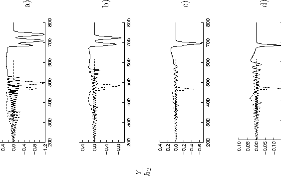
linear shallow water speed of the two-fluid system. The resulting profiles
of the interface exhibit an undular depression that is developing ahead
of the body, with a number of oscillations which is increasing with time,
see figure 1. Behind the body an almost horizontal
elevation develops, with length which also is increasing with time. We
find that the results in figure 1 are typical for
speed of the body in the interval 0.38<
U/c0<1.02,
approximately, for this configuration. The lower limit corresponds to the
lower limit of the transcritical regime.
g cm-3. A body, starting from rest, is moving horizontally with
speed U in the upper layer, and we shall compute the resulting motion
of the interface. The shape of the body is determined by y=h2-H0sech2(Kx),
where H0=0.4h2
and KH0=0.1989. This
configuration corresponds to a set of experiments described by Melville
& Helfrich (1987). (We have been able to simulate their experiments
with good agreement using the present fully nonlinear method, where weakly
nonlinear KdV-theory exhibits severe shortcomings). First we consider two
examples where the speed of the body is either U=0.81c0
or U=0.94c0, where c0 in the
linear shallow water speed of the two-fluid system. The resulting profiles
of the interface exhibit an undular depression that is developing ahead
of the body, with a number of oscillations which is increasing with time,
see figure 1. Behind the body an almost horizontal
elevation develops, with length which also is increasing with time. We
find that the results in figure 1 are typical for
speed of the body in the interval 0.38<
U/c0<1.02,
approximately, for this configuration. The lower limit corresponds to the
lower limit of the transcritical regime.
Solitary waves
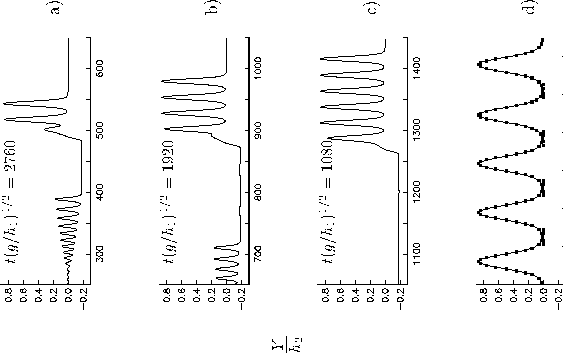
In the next example we consider the same problem as above, but let the body have speed U/c0=1.09. Now we also want to vary the thickness of the body, to investigate the effect of various forcing. In the first case (figure 3a) the thickness of the body is H0=0.4h2. Now the moving body generates a train of solitary waves propagating upstream, with an amplitude a=1.171h2. We have compared the saturated leading waves with fully nonlinear solitary wave solutions of the corresponding steady problem, with a very high agreement (see also figure 4d for another example).
We then halve the thickness of the body ( H0=0.2h2) and display results in figure 3b. The generated solitary waves have now somewhat reduced amplitude and generation rate as compared to the previous example. The reduction of the body thickness is once more repeated (figure 3c), i.e. H0=0.1h2, but still upstream solitary waves are generated, now with a quite reduced generation rate, however. When the height of the body is reduced still more, to H0=0.05h2, solitary waves are not generated. The flow becomes supercritical, with a minor depression moving with the same speed as the body (figure 3d).
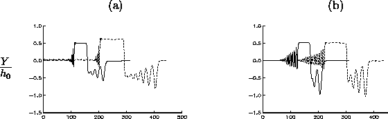
In another example the two-fluid system at rest has thicknesses h1
and h2=4h1 (a thin layer below a thick)
and ratio between the densities ![]() .
A half-elliptical body with horizontal and vertical half-axes 10h1and
0.1h1, respectively, is moving horizontally with speed
U=1.1c0
along the bottom of the lower (thinner) layer. This geometry has approximately
the same volume as the former one but is more slender, and therefore imposes
weaker nonlinearity on the problem. Still upstream solitary waves with
height of the order of the thinner layer are generated, see figure
4.
.
A half-elliptical body with horizontal and vertical half-axes 10h1and
0.1h1, respectively, is moving horizontally with speed
U=1.1c0
along the bottom of the lower (thinner) layer. This geometry has approximately
the same volume as the former one but is more slender, and therefore imposes
weaker nonlinearity on the problem. Still upstream solitary waves with
height of the order of the thinner layer are generated, see figure
4.
For both geometries we have found that solitary waves are generated
for a rather narrow interval of the speed, i.e. 1.05<U/c0<1.15,
approximately. The generated solitary waves have always an amplitude comparable
to the depth of the thinner layer.
Topography in the thicker layer
We have also performed some simulations for a body moving horizontally with constant speed in the thicker of the two layers (results not shown). If the lower layer is the thicker one, a depression of the interface develops behind the body. This depression may be rather significant, depending on the size of the body. Correspondingly, the interface is lifted upstream of the body. We have not observed that waves are generated upstream for this configuration.
Another interesting problem, which we have not yet investigated, is
that with an oscillatory flow at stationary body, which is relevant to
tidal driven flow at a bottom topography. We aim to perform simulations
for this problem and present the results at the workshop.
Comparison with experiments
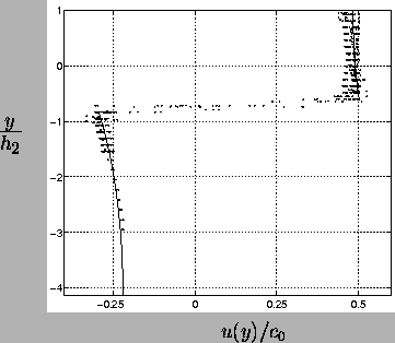
In the ocean (or in the atmosphere) the density profile is seldom very sharp, and one may question the relevance of a two-layer model where two homogeneous fluids are separeted by a sharp interface. On the otherhand, if an infinitely sharp pycnocline could be created in nature, one would expect any wave motion to break up due to the Kelvin-Helmholtz instability. In order to investigate these issues we have performed several experiments in a wave tank on internal solitary waves. The solitary waves may propagate along a pycnocline separating a thinner layer of fresh water above a thicker layer of brine. The thickness of the pycnocline is in the interval 0.13 - 0.26 times the depth of the thinner layer, approximately. The induced fluid velocities are measured quite accurately using Particle Tracking Velocimetry. In figure 2 we show an example of the velocity profile at the crest of a solitary wave. Data from several experiments are included. Also is shown a comparison with the fully nonlinear theory, with good agreement. We have performed several other experiments, also with good agreement with theory (results may be found in reference 2). We have observed that Kelvin-Helmholtz instability only occurs for the largest waves (close to the maximal amplitude). Instability appears to occur according to the theorem of Miles and Howard.
This research was supported by The Research Council of Norway.
References
GRUE, J., FRIIS, H. A., PALM, E. AND RUSåS, P. O. A method for computing unsteady fully nonlinear interfacial waves. J. Fluid Mech., 351, 1997.
GRUE, J., JENSEN, A., RUSåS,
P.
O. AND SVEEN, J. K. Properties
of large amplitude internal waves. J. Fluid Mech. (to appear). 1998.
 |